CNN on CIFAR10 Data set using PyTorch
The goal is to apply a Convolutional Neural Net Model on the CIFAR10 image data set and test the accuracy of the model on the basis of image classification.
CIFAR10 is a collection of images used to train Machine Learning and Computer Vision algorithms. It contains 60K images having dimension of 32x32 with ten different classes such as airplanes, cars, birds, cats, deer, dogs, frogs, horses, ships, and trucks. We train our Neural Net Model specifically Convolutional Neural Net (CNN) on this data set.
CNN's are a class of Deep Learning Algorithms that can recognize and and classify particular features from images and are widely used for analyzing visual images.
There are two main parts to a CNN architecture
- A convolution tool that separates and identifies the various features of the image for analysis in a process called as Feature Extraction.
- A fully connected layer that utilizes the output from the convolution process and predicts the class of the image based on the features extracted in previous stages.
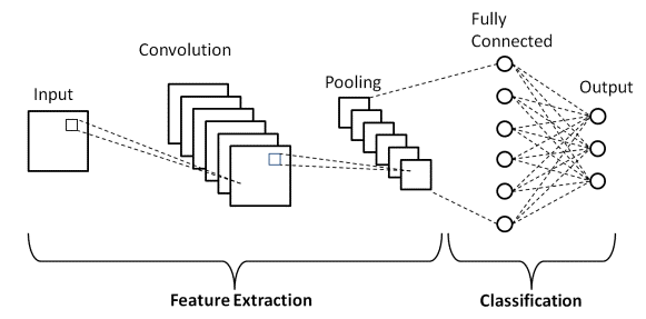
There are mainly three types of layers:
- Convolutional Layer : Used to extract features from the image. It creates an MxM matrix filter that slides over the image and uses dot product with the input of the image. This gives us a Feature Map that gives us information about the image such as corners, edges. This is then fed to the other layers to learn more about the image.
- Pooling Layer : The main goal of this layer is to reduce the convoluted size of the feature map and to reduce Computational costs. This is done by decreasing the connections between layers. It acts as a bridge between Convolutional Layer and the FC layer.
- Fully Connected Layer : This layer consists of weights and biases along with neurons to connect the various layers. The input image is flattened and fed to this layer. Mathematical operations are then used to do classification of images.
- Dropout Layer : Usually when all features are connected to FC Layer, it can cause over fitting wherein model performs well on training set but not on the test set. On passing a dropout of 0.3, 30% of neurons are dropped randomly from the network
- Activation Functions : These are used to learn and approximate any kind of continuous and complex relations between variables of the network. It decides when the variables should fire and when they shouldn't. It also adds non-linearity to the model.
In our example we start by importing the required packages
import torchimport numpy as npfrom torchvision import datasetsimport torchvision.transforms as transformsfrom torch.utils.data.sampler import SubsetRandomSampler
Since these are large images (32x32x3), we use GPU to train our model so that it is much faster.
import torch
import numpy as np

# check if CUDA is available
train_on_gpu = torch.cuda.is_available()

if not train_on_gpu:
    print('CUDA is not available.  Training on CPU ...')
else:
    print('CUDA is available!  Training on GPU ...')
Next we load the CIFAR10 Data set
from torchvision import datasets
import torchvision.transforms as transforms
from torch.utils.data.sampler import SubsetRandomSampler

# number of subprocesses to use for data loading
num_workers = 0
# how many samples per batch to load
batch_size = 20
# percentage of training set to use as validation
valid_size = 0.2

# convert data to a normalized torch.FloatTensor
transform = transforms.Compose([
    transforms.ToTensor(),
    transforms.Normalize((0.5, 0.5, 0.5), (0.5, 0.5, 0.5))
    ])

# choose the training and test datasets
train_data = datasets.CIFAR10('data', train=True,
                              download=True, transform=transform)
test_data = datasets.CIFAR10('data', train=False,
                             download=True, transform=transform)

# obtain training indices that will be used for validation
num_train = len(train_data)
indices = list(range(num_train))
np.random.shuffle(indices)
split = int(np.floor(valid_size * num_train))
train_idx, valid_idx = indices[split:], indices[:split]

# define samplers for obtaining training and validation batches
train_sampler = SubsetRandomSampler(train_idx)
valid_sampler = SubsetRandomSampler(valid_idx)

# prepare data loaders (combine dataset and sampler)
train_loader = torch.utils.data.DataLoader(train_data, batch_size=batch_size,
    sampler=train_sampler, num_workers=num_workers)
valid_loader = torch.utils.data.DataLoader(train_data, batch_size=batch_size,
    sampler=valid_sampler, num_workers=num_workers)
test_loader = torch.utils.data.DataLoader(test_data, batch_size=batch_size,
    num_workers=num_workers)

# specify the image classes
classes = ['airplane', 'automobile', 'bird', 'cat', 'deer',
           'dog', 'frog', 'horse', 'ship', 'truck']
We try and visualize the data set in order to do feature extraction
import matplotlib.pyplot as plt
%matplotlib inline

# helper function to un-normalize and display an image
def imshow(img):
    img = img / 2 + 0.5  # unnormalize
    plt.imshow(np.transpose(img, (1, 2, 0)))  # convert from Tensor image# obtain one batch of training images
dataiter = iter(train_loader)
images, labels = dataiter.next()
images = images.numpy() # convert images to numpy for display# plot the images in the batch, along with the corresponding labels
fig = plt.figure(figsize=(25, 4))# display 20 images
for idx in np.arange(20):
ax = fig.add_subplot(2, 20/2, idx+1, xticks=[], yticks=[])
imshow(images[idx])
ax.set_title(classes[labels[idx]])

View the images in more detail. Here, we look at the normalized red, green, and blue (RGB) color channels as three separate, grayscale intensity images.
rgb_img = np.squeeze(images[19])
channels = ['red channel', 'green channel', 'blue channel']

fig = plt.figure(figsize = (36, 36))
for idx in np.arange(rgb_img.shape[0]):
    ax = fig.add_subplot(1, 3, idx + 1)
    img = rgb_img[idx]
    ax.imshow(img, cmap='gray')
    ax.set_title(channels[idx])
    width, height = img.shape
    thresh = img.max()/2.5
    for x in range(width):
        for y in range(height):
            val = round(img[x][y],2) if img[x][y] !=0 else 0
            ax.annotate(str(val), xy=(y,x),
                    horizontalalignment='center',
                    verticalalignment='center', size=8,
                    color='white' if img[x][y]<thresh else 'black')
To compute the output size of a given convolutional layer we can perform the following calculation (taken from Stanford’s cs231n course):
We can compute the spatial size of the output volume as a function of the input volume size (W), the kernel/filter size (F), the stride with which they are applied (S), and the amount of zero padding used (P) on the border. The correct formula for calculating how many neurons define the output_W is given by (W−F+2P)/S+1.
For example for a 7x7 input and a 3x3 filter with stride 1 and pad 0 we would get a 5x5 output. With stride 2 we would get a 3x3 output.
import torch.nn as nn
import torch.nn.functional as F# define the CNN architecture
class Net(nn.Module):  def __init__(self):
    super(Net, self).__init__()
    self.conv1 = nn.Conv2d(3, 6, 5)
    self.pool = nn.MaxPool2d(2, 2)
    self.conv2 = nn.Conv2d(6, 16, 5)
    self.fc1 = nn.Linear(16 * 5 * 5, 120)
    self.fc2 = nn.Linear(120, 84)
    self.fc3 = nn.Linear(84, 10)  def forward(self, x):
    x = self.pool(F.relu(self.conv1(x)))
    x = self.pool(F.relu(self.conv2(x)))
    x = x.view(-1, 16 * 5 * 5)
    x = F.relu(self.fc1(x))
    x = F.relu(self.fc2(x))
    x = self.fc3(x)
    return x# create a complete CNN
model = Net()
print(model)# move tensors to GPU if CUDA is available
if train_on_gpu:
model.cuda()

Using a Loss Function and Optimization function. These help us in calculating the difference between the actual output and the target variable. Here we will be using SGD (Stochastic Gradient Descent) optimizer. The gradient descent helps us in reducing losses over time. This is heavily influenced by the learning rate. Learning rate helps us how quickly the model converges to the solution. Here we have chosen a value of 0.01
import torch.optim as optim# specify loss function
criterion = nn.CrossEntropyLoss()# specify optimizer
optimizer = optim.SGD(model.parameters(), lr=.01)
Now we train our model using Validation set. It is used to see how our model performs before using the actual testing set.
We need to take a close look at our validation set losses. If the losses increase then it is a case of overfitting
# number of epochs to train the model
n_epochs = [*range(30)]#List to store loss to visualize
train_losslist = []valid_loss_min = np.Inf # track change in validation loss

for epoch in range(1, n_epochs+1):

    # keep track of training and validation loss
    train_loss = 0.0
    valid_loss = 0.0

    ###################
    # train the model #
    ###################
    model.train()
    for data, target in train_loader:
        # move tensors to GPU if CUDA is available
        if train_on_gpu:
            data, target = data.cuda(), target.cuda()
        # clear the gradients of all optimized variables
        optimizer.zero_grad()
        # forward pass: compute predicted outputs by passing inputs to the model
        output = model(data)
        # calculate the batch loss
        loss = criterion(output, target)
        # backward pass: compute gradient of the loss with respect to model parameters
        loss.backward()
        # perform a single optimization step (parameter update)
        optimizer.step()
        # update training loss
        train_loss += loss.item()*data.size(0)

    ######################
    # validate the model #
    ######################
    model.eval()
    for data, target in valid_loader:
        # move tensors to GPU if CUDA is available
        if train_on_gpu:
            data, target = data.cuda(), target.cuda()
        # forward pass: compute predicted outputs by passing inputs to the model
        output = model(data)
        # calculate the batch loss
        loss = criterion(output, target)
        # update average validation loss
        valid_loss += loss.item()*data.size(0)

    # calculate average losses
    train_loss = train_loss/len(train_loader.dataset)
    valid_loss = valid_loss/len(valid_loader.dataset)    train_losslist.append(train_loss)

    # print training/validation statistics
    print('Epoch: {} \tTraining Loss: {:.6f} \tValidation Loss: {:.6f}'.format(
        epoch, train_loss, valid_loss))

    # save model if validation loss has decreased
    if valid_loss <= valid_loss_min:
        print('Validation loss decreased ({:.6f} --> {:.6f}).  Saving model ...'.format(
        valid_loss_min,
        valid_loss))
        torch.save(model.state_dict(), 'model_cifar.pt')
        valid_loss_min = valid_lossplt.plot(n_epochs, train_losslist)
plt.xlabel("Epoch")
plt.ylabel("Loss")
plt.title("Performance of Model 1")
plt.show()
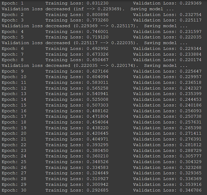

Now loading the model with the lowest Validation loss value
model.load_state_dict(torch.load('model_cifar.pt'))
Now we test the model on a testing set
# track test loss
test_loss = 0.0
class_correct = list(0. for i in range(10))
class_total = list(0. for i in range(10))

model.eval()
# iterate over test data
for data, target in test_loader:
    # move tensors to GPU if CUDA is available
    if train_on_gpu:
        data, target = data.cuda(), target.cuda()
    # forward pass: compute predicted outputs by passing inputs to the model
    output = model(data)
    # calculate the batch loss
    loss = criterion(output, target)
    # update test loss
    test_loss += loss.item()*data.size(0)
    # convert output probabilities to predicted class
    _, pred = torch.max(output, 1)
    # compare predictions to true label
    correct_tensor = pred.eq(target.data.view_as(pred))
    correct = np.squeeze(correct_tensor.numpy()) if not train_on_gpu else np.squeeze(correct_tensor.cpu().numpy())
    # calculate test accuracy for each object class
    for i in range(batch_size):
        label = target.data[i]
        class_correct[label] += correct[i].item()
        class_total[label] += 1

# average test loss
test_loss = test_loss/len(test_loader.dataset)
print('Test Loss: {:.6f}\n'.format(test_loss))

for i in range(10):
    if class_total[i] > 0:
        print('Test Accuracy of %5s: %2d%% (%2d/%2d)' % (
            classes[i], 100 * class_correct[i] / class_total[i],
            np.sum(class_correct[i]), np.sum(class_total[i])))
    else:
        print('Test Accuracy of %5s: N/A (no training examples)' % (classes[i]))

print('\nTest Accuracy (Overall): %2d%% (%2d/%2d)' % (
    100. * np.sum(class_correct) / np.sum(class_total),
    np.sum(class_correct), np.sum(class_total)))
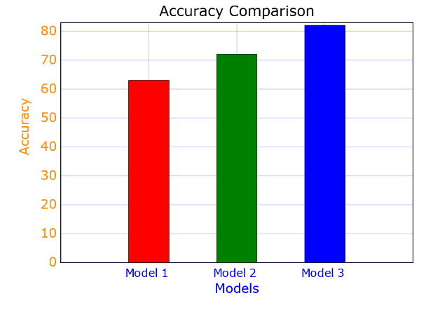
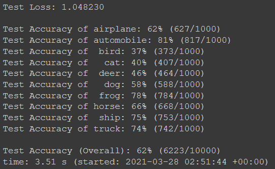
We can see that we get an accuracy of 63% if we use the model given in the PyTorch tutorial which is pretty bad. We need to tweak the model as well as the hyper parameters to get a better score
My first attempt was using a sequential CNN that has more layers and a larger batch size along with defined flattening layer.
class Net(nn.Module):
    def __init__(self):
        super(Net, self).__init__()
        # convolutional layer
        self.conv1 = nn.Conv2d(3, 16, 3, padding=1)
        self.conv2 = nn.Conv2d(16, 32, 3, padding=1)
        self.conv3 = nn.Conv2d(32, 64, 3, padding=1)
        # max pooling layer
        self.pool = nn.MaxPool2d(2, 2)
        # fully connected layers
        self.fc1 = nn.Linear(64 * 4 * 4, 512)
        self.fc2 = nn.Linear(512, 64)
        self.fc3 = nn.Linear(64, 10)
        # dropout
        self.dropout = nn.Dropout(p=.5)

    def forward(self, x):
        # add sequence of convolutional and max pooling layers
        x = self.pool(F.relu(self.conv1(x)))
        x = self.pool(F.relu(self.conv2(x)))
        x = self.pool(F.relu(self.conv3(x)))
        # flattening
        x = x.view(-1, 64 * 4 * 4)
        # fully connected layers
        x = self.dropout(F.relu(self.fc1(x)))
        x = self.dropout(F.relu(self.fc2(x)))
        x = self.fc3(x)
        return x


After testing this model we can see an increase in our accuracy

The channels have been set as 3 and 16 for the first Conv Layer. 16 and 32 for next layer and then 32 and 64 for third layer. Channels are matrices that are used in the dot product when doing feature selection.
Next is changes in Maxpool Layer. This down samples the input representation by taking the maximum value over the window defined by pool size for each dimension along the features axis.
It also includes a 50% dropout layer to reduce over fitting.
These changes led us to an increase in accuracy to 72%.
To increase the accuracy, we need to tweak hyper parameters more along with the learning rate.
class CNN(nn.Module):


    def __init__(self):

        super(CNN, self).__init__()

        self.conv_layer = nn.Sequential(

            # Conv Layer block 1
            nn.Conv2d(in_channels=3, out_channels=32, kernel_size=3, padding=1),
            nn.BatchNorm2d(32),
            nn.ReLU(inplace=True),
            nn.Conv2d(in_channels=32, out_channels=64, kernel_size=3, padding=1),
            nn.ReLU(inplace=True),
            nn.MaxPool2d(kernel_size=2, stride=2),

            # Conv Layer block 2
            nn.Conv2d(in_channels=64, out_channels=128, kernel_size=3, padding=1),
            nn.BatchNorm2d(128),
            nn.ReLU(inplace=True),
            nn.Conv2d(in_channels=128, out_channels=128, kernel_size=3, padding=1),
            nn.ReLU(inplace=True),
            nn.MaxPool2d(kernel_size=2, stride=2),
            nn.Dropout2d(p=0.05),

            # Conv Layer block 3
            nn.Conv2d(in_channels=128, out_channels=256, kernel_size=3, padding=1),
            nn.BatchNorm2d(256),
            nn.ReLU(inplace=True),
            nn.Conv2d(in_channels=256, out_channels=256, kernel_size=3, padding=1),
            nn.ReLU(inplace=True),
            nn.MaxPool2d(kernel_size=2, stride=2),
        )


        self.fc_layer = nn.Sequential(
            nn.Dropout(p=0.1),
            nn.Linear(4096, 1024),
            nn.ReLU(inplace=True),
            nn.Linear(1024, 512),
            nn.ReLU(inplace=True),
            nn.Dropout(p=0.1),
            nn.Linear(512, 10)
        )


    def forward(self, x):
        """Perform forward."""

        # conv layers
        x = self.conv_layer(x)

        # flatten
        x = x.view(x.size(0), -1)

        # fc layer
        x = self.fc_layer(x)

        return x
Here I increased the amount of layers, added Convolutional blocks that have a kernel size of 3. A kernel is a filter used to extract features from the images. I also changed the channel sizes.
Next thing I did is change the learning rate from 0.01 to 0.001 so that our model converges more gradually.
import torch.optim as optim# specify loss function
criterion = nn.CrossEntropyLoss()# specify optimizer
optimizer = optim.SGD(model.parameters(), lr=.001)
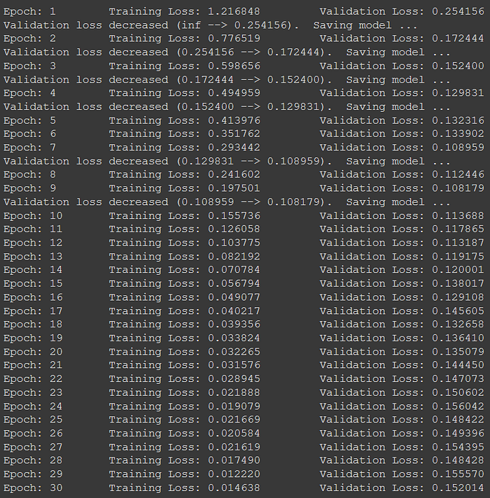

We get accuracy output as

We can see that our accuracy drastically improved to 82%. This happens because the batch sizes in the previous models were too small for the data set which is quite large. Next, our learning rate was set at a higher value thus we were not able to reach the minimum loss in 30 epochs. Changing it to 0.001 helps us converge much more quickly.
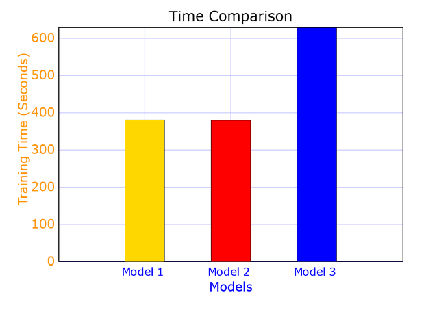
Comparison between the models
Challenges faced
- Feature extraction is an issue. The model struggles when multiple colors are involved in the image. It struggles for images of cats, dogs and birds which are multicolored as compared to the other objects
- Tried running the model for greater number of epochs and with a much lower learning rate. This caused over fitting and drastically reduced the accuracy of the model

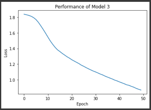
3. The tuning of hyper parameters is a challenging task since the training of the models takes a long time.
References
- https://pytorch.org/tutorials/beginner/blitz/cifar10_tutorial.html#sphx-glr-beginner-blitz-cifar10-tutorial-py
- https://www.upgrad.com/blog/basic-cnn-architecture/
- https://www.kaggle.com/datajameson/cifar-10-object-recognition-cnn-explained
- https://zhenye-na.github.io/2018/09/28/pytorch-cnn-cifar10.html
- https://www.stefanfiott.com/machine-learning/cifar-10-classifier-using-cnn-in-pytorch/
- https://medium.com/swlh/image-classification-with-cnn-4f2a501faadb
- https://github.com/martinoywa/cifar10-cnn-exercise/blob/master/cifar10_cnn_exercise.ipynb
